Can Math Alone Prove Guilt?
The Couple Who Looked Guilty — by Numbers

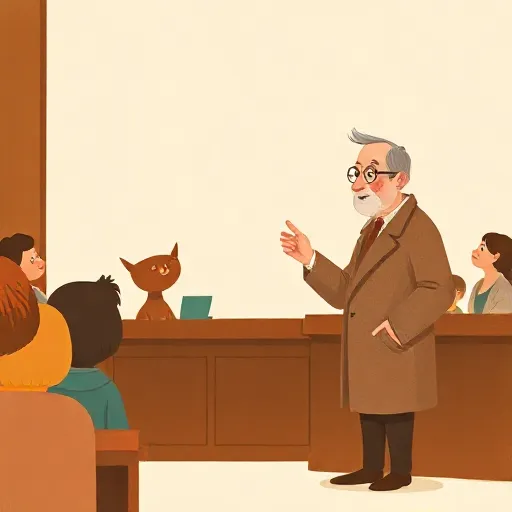
In 1964 Los Angeles, a married couple, Janet and Malcolm Collins, stood trial for robbery. An eyewitness described a black man with a beard and a mustache, a white woman with blonde hair in a ponytail, and a yellow convertible — an interracial couple. A college mathematician took the stand. He assigned a probability to each feature: a black man with a beard 1 in 10, man with a mustache 1 in 4, white woman with blond hair 1 in 3, woman with a ponytail 1 in 10, interracial couple in a car 1 in 1000, yellow convertible 1 in 10. Multiplying them, he testified the chance of a random couple matching all six was 1 in 12 million. The jury convicted.
The California Supreme Court later reversed the conviction. The judges spotted two huge mistakes. First, the mathematician assumed the features were independent — that having a beard told you nothing about having a mustache. But beards and mustaches often go together. Blonde hair and a ponytail are also linked. Multiplying probabilities only works if the events have nothing to do with each other. Second, even if the 1-in-12-million figure were correct, it didn’t mean the Collins were guilty. It meant only this: if they were innocent, the chance they’d still match the description was 1 in 12 million. That’s not at all the same as the chance they were innocent given the match. Juries, and sometimes experts, mix these up all the time.
What’s the Chance You’re Guilty? The Prosecutor’s Fallacy
This mix-up has a name: the prosecutor’s fallacy. It happens when someone treats the probability of the evidence assuming the defendant is innocent as if it were the probability the defendant is innocent given the evidence. The two are different because of conditional probability — the chance of A when B is true isn’t the same as the chance of B when A is true.
Imagine a test for a rare disease. Suppose the test is 99% accurate: if you have the disease, the test will say yes 99% of the time. But if you don’t have it, the test still says yes 5% of the time (a false positive). Now you test positive. What’s the chance you actually have the disease? Not 95%. The disease is rare — only 1 in 1,000 people have it. So before the test, your prior probability of having it is 0.001. Using a rule called Bayes’ theorem, which combines prior beliefs with new evidence, your chance of truly having the disease after a positive test turns out to be about 2%, not 95%. Ignoring the base rate — how common the disease is — leads to the base rate fallacy.
The same logic applies to courtrooms. An expert might testify that a bloodstain matches the defendant and that only 5% of random people would match by coincidence. That 5% is the chance of a match if the defendant were innocent. It is not the chance the defendant is innocent given a match. To get that, you need the prior probability that the defendant was the source. If, before any evidence, the defendant was just one of 10,000 possible suspects, the prior chance they were the source is 1 in 10,000. After a match with a 5% random-match probability, the chance the defendant is the source rises — but only to about 0.2%, not 95%. Missing the prior leads you wildly astray.
How Strong Is a Clue? Likelihood Ratios and Bayes’ Theorem

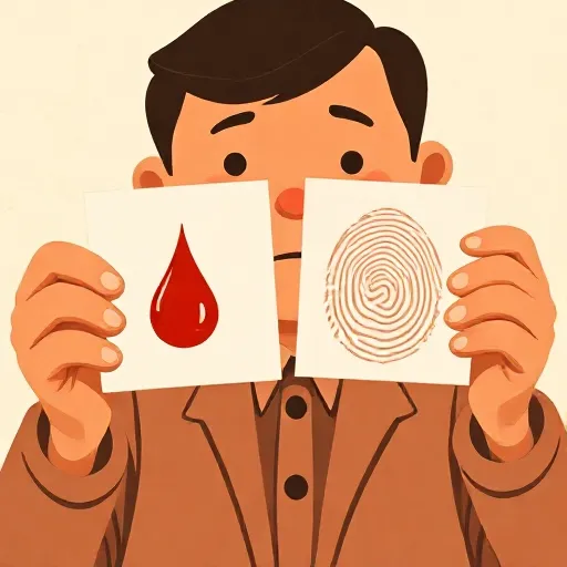
Legal probabilists — scholars like David Kaye (b. 1947) and Richard Lempert — argue that probability theory can still help, if used carefully. Instead of focusing on a single number like a posterior probability, they look at the likelihood ratio. This ratio compares how probable the evidence is under two competing stories: the prosecutor’s hypothesis and the defense’s hypothesis.
Say the evidence is a DNA match. The likelihood ratio is: probability of the match if the defendant was the source, divided by the probability of the match if a random innocent person was the source. If the defense story is that an unknown person left the stain, and the random-match probability is 1 in 100 million, the numerator is near 1 (the test will almost certainly match if the defendant is the source), so the likelihood ratio is about 100 million. That’s strong evidence. It doesn’t tell you the final chance of guilt — you still need a prior — but it tells you how much the evidence should shift your belief.
Using the odds form of Bayes’ theorem, you multiply the prior odds by the likelihood ratio to get the posterior odds. This structure helps courts avoid the prosecutor’s fallacy. It also shows that a piece of evidence can be very strong even if the final probability of guilt stays modest — because the prior was extremely low.
When the Numbers Point Everywhere: Naked Statistics

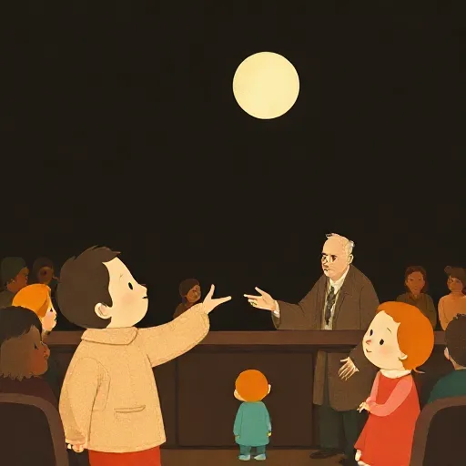
Probability run crisply can still land us in puzzles. In 1971, the legal scholar Laurence Tribe (b. 1941) asked: Suppose a woman is hit by a bus, but she is color-blind and can’t tell whether it was a Blue Bus or a Red Bus. In that town, 80% of buses are Blue Bus company’s. So the probability that a Blue Bus hit her is 80% — well above the 50% threshold in civil cases. Yet most courts would not let her win a lawsuit against Blue Bus on that statistic alone. This is the Blue Bus case, an example of naked statistical evidence.
Another classic is the Gatecrasher: 1,000 people attend a rodeo, but only 499 bought tickets. For any spectator picked at random, the chance they gatecrashed is just over 50%. Still, you can’t point to someone in the stands and sue them solely because they belong to that group. A third puzzle is the Prisoner: 100 prisoners are in a yard; 99 attack and kill a guard, one does nothing. If you pick one prisoner at random, the probability he is guilty is 99%. Yet most people feel you can’t convict him beyond a reasonable doubt without something that ties the act to him personally.
These examples bother legal probabilists because the numbers cross the required probability thresholds — 50% for civil cases, perhaps 90‑95% for criminal ones — but the evidence doesn’t feel like proof. Philosophers like L. Jonathan Cohen (1923–2006) argued that such paradoxes show probability alone can’t be the whole story about legal proof.
The Conjunction Paradox: When Adding Details Weakens the Case

Cohen raised another objection, the conjunction paradox. In a lawsuit, a plaintiff often has to prove several things. Suppose you must prove two separate claims — say, that the defendant was driving the car and that they were drunk. Under a “preponderance of the evidence” standard, you need each claim to be more likely than not, above 50%. Now imagine each claim is proven with a probability of 70%. Most people think you’ve met the standard for both. Yet if the two claims are independent, the probability that both are true is 0.7 × 0.7 = 0.49, or 49% — below the 50% line. The law seems to say “prove each element to 50%” but the probability of the whole case can fall below 50%.
Legal probabilists have proposed several fixes. Some say that what matters is the comparative probability of the plaintiff’s entire story against the defendant’s entire story, not splitting it into independent elements. Others suggest that the standard should be defined by likelihood ratios rather than posterior probabilities, though that approach brings its own puzzles. Still, the conjunction paradox reminds us that merging evidence probabilistically isn’t as simple as adding up scores.
Why the Law Still Argues About Numbers

Probability has undeniable power: it catches fallacies, helps compare rival stories, and clarifies the difference between weak and strong evidence. Yet the puzzles of naked statistics and conjunction show that slapping a number on a verdict isn’t enough. Courts still debate how to handle DNA cold-hit cases — where a suspect is found solely through a database search — because they look eerily like the Prisoner puzzle. The concept of reference classes adds further trouble: when we say the chance a defendant committed a crime is, say, 0.2% because he is a Nigerian drug courier, we are picking one group among many possible groups he belongs to. Is that the right group? Why not toll collectors at the George Washington Bridge? Even statisticians disagree.
What does this mean for you? Every day you weigh evidence: whether a friend’s excuse is true, whether a social media post is reliable. You’re already using rough probabilities. But the legal debate shows that pure numbers can feel unfair or incomplete when they don’t connect to a specific person’s actions. The tension between cold math and individualized justice is not just a lawyer’s problem — it’s a puzzle about how any of us should balance statistics with stories when making serious decisions.
Think about it
- If a DNA database search points to one person among a million with a 1-in-100-million match, but there is no other evidence, would you feel confident convicting them? Why or why not?
- In the Gatecrasher case, what if the organizers could choose to sue only people who had previously skipped paying at other events — would that change your view? What information should count as “individualized”?
- Suppose two friends tell you different versions of what happened at a party, and each story has some unlikely details. How would you go about combining the clues without making a prosecutor’s fallacy in your own head?